Extreme sparsity gives rise to functional specialization
Modularity of neural networks – both biological and artificial – can be thought of either structurally or functionally, and the relationship between these is an open question. We show that enforcing structural modularity via sparse connectivity between two dense sub-networks which need to communicate to solve the task leads to functional specialization of the sub-networks, but only at extreme levels of sparsity. With even a moderate number of interconnections, the sub-networks become functionally entangled. Defining functional specialization is in itself a challenging problem without a universally agreed solution. To address this, we designed three different measures of specialization (based on weight masks, retraining and correlation) and found them to qualitatively agree. Our results have implications in both neuroscience and machine learning. For neuroscience, it shows that we cannot conclude that there is functional modularity simply by observing moderate levels of structural modularity: knowing the brain’s connectome is not sufficient for understanding how it breaks down into functional modules. For machine learning, using structure to promote functional modularity – which may be important for robustness and generalization – may require extremely narrow bottlenecks between modules.
Introduction
Modularity of neural networks is a bit like the notion of beauty in art: everyone agrees that it’s important, but nobody can say exactly what it means. Modularity has been widely observed in the brain (Mountcastle 1997; Sporns, Tononi, and Kötter 2005; Chen et al. 2008; Meunier et al. 2009), suggested to be important in evolution (Redies and Puelles 2001; Clune, Mouret, and Lipson 2013; Kashtan and Alon 2005) and learning (Ellefsen, Mouret, and Clune 2015), and found in trained artificial neural networks (Filan et al. 2021). One definition is that a network is modular if it can be broken down into composable subnetworks that can operate independently (Amer and Maul 2019). This definition has a structural and functional component. Structural, because we partition neurons in the network into different modules. Functional, because these modules are then required to carry out independent functions.
Structural notions of modularity can be easily measured by constructing a graph of neurons as nodes and synapses as edges (Bullmore and Bassett 2011), for example the \(Q\) modularity measure of how many edges are within modules compared to between modules (Newman 2006). Functional measures of modularity are much less straightforward. How can you quantitatively measure whether a sub-network is independent or composable? Do different proposed measures of functional modularity agree? Do they agree with a structural measure?
We investigate these questions with a simple network architecture and set of tasks designed to allow us to control the degree of structural modularity. We then compare different measures of functional specialization of these modules to certain sub-tasks. Reassuringly, we find that the three functional measures qualitatively agree. However, we also find that only extreme levels of structural modularity give rise to functional modularity. These results can serve as a guideline for the design of artificial neural networks that want to introduce functional modularity. However, they may also pose difficulties for the interpretation of biological, connectomic data, since our results imply that even relatively strong structural modularity may have no functional bearing (Sporns, Tononi, and Kötter 2005).
We describe the architecture and tasks in 2, the measures of functional specialization in 3, and the results of our experiments in 4. We discuss the implications and limitations of these results in 5.
Architecture and tasks
Our approach to investigating the relationship between structural and functional modularity is to explicitly design a network with a controllable degree of structural modularity. We then train it on a task designed to be composed of clearly defined sub-tasks, and measure the degree of functional modularity in the trained network. The simplest possible network that could be described as modular would have only two modules. Therefore, our architecture consists of two sub-networks, each one being densely and recurrently connected. We add sparse interconnections between neurons in these two sub-networks, with a degree of sparsity ranging from a single connection in each direction between the sub-networks, right up to dense inter-connectivity. With dense inter-connectivity, the network ceases to be structurally modular as every neuron is connected to every other neuron. Each sub-network receives an MNIST digit (LeCun and Cortes 2010) as input, and the task is to return one digit or the other depending on whether the parity of the two digits is the same or different. With this task, the two networks are required to communicate, but are able to specialize in recognizing their own digit because it is sufficient to communicate only the parity of their own digit to the other sub-network.
In this section we describe the architecture, tasks and training in more detail. In 3 we describe the measures of functional modularity.
Tasks
We designed a nested task to allow us to measure functional specialization of sub-networks.
Sub-network \(j\) receives as input an instance of digit \(D_j \in \left\{0, ..., 9\right\}\). We define the parity difference as \(P=(D_0+D_1)\bmod 2\). The value of \(P\) is 0 if the parity of the two digits is the same, or 1 if it is different. The network needs to return digit 0 if the parity is the same, or digit 1 if different. Solving this task requires only communicating a single parity bit between the sub-networks. \[\label{eq:parity-difference-task} \mathrm{Target}=PD_0+(1-P)D_1\]
The sub-tasks are to predict only one of the input digits. \[\label{eq:sub-task} \mathrm{Target}_k=D_k, \quad k \in \left\{0, 1\right\}\]
Note that we exclude the case \(D_0=D_1\) because the target is then ambiguous. This case has parity difference \(P=0\). To resolve the imbalance in the distribution of parity differences, we also exclude one case where the parity difference is \(P=1\) by requiring \(D_1-D_0\bmod 10\neq 1\). We combine these two exclusions by requiring that \((D_1-D_0)\bmod 10\not\in\{0,1\}\).
Architectures
The network consists of two dense recurrent sub-networks each receiving their own separate input, with sparse connections between the two sub-networks (1). Each sub-network \(n \in \left\{0, 1\right\}\) is composed of a single hidden layer \(\textbf{h}^{(n)}\) of \(N=100\) neurons, receiving input through weights \(W^{(n)}_{ih}\) and bias \(\beta^{(n)}_{ih}\) and recurrently connected through weights \(W^{(n)}_{hh}\) and bias \(\beta^{(n)}_{hh}\). The two sub-networks are then connected through sparse weights \(W_{sparse}^{0\xrightarrow{}1}\), \(W_{sparse}^{1\xrightarrow{}0}\).
[fig:architecture]
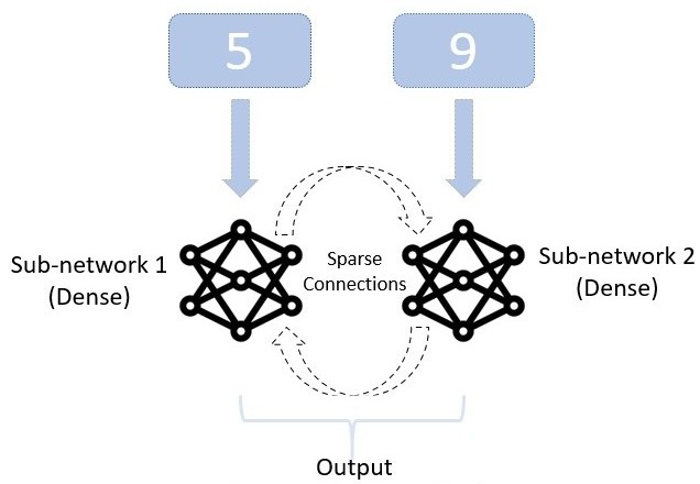
The digits are presented for \(T=5\) time steps. Each sub-network is presented with an input \(x^{(n)}\). We write \(m=1-n\) to be the index of the other sub-network. The hidden state \(h_t^{(n)}\) of sub-network \(n \in \left\{0, 1\right\}\) at time-step \(t\) is then: \[h_t^{(n)} = \tanh\left( W^{(n)}_{ih} x^{(n)} + \beta^{(n)}_{ih} + W^{(n)}_{hh} h_{t-1}^{(n)} + \beta^{(n)}_{hh} + W_{sparse}^{m\xrightarrow{}n}h_{t-1}^{(m)} \right).\]
Note that this formulation could be easily adapted for other types of sub-networks like LSTMs (Sak, Senior, and Beaufays 2014) or leaky RNN cells.
Each sub-network is densely connected to a readout layer \(\mathbf{r}^{(n)}\) through weights \(W^{(n)}_{hr}\) and bias \(\beta^{(n)}_{hr}\): \[\mathbf{r}^{(n)}=W^{(n)}_{hr}\mathbf{h}^{(n)}_T+\beta^{(n)}_{hr}.\] Given the two readouts layer, we compute the actual decision of the global model using a competitive max decision. For each input sample, the sub-network with the highest “certainty” (largest value) takes the decision. The output layer of the whole network \(\mathbf{r}^{out}\) is defined to be the output layer of the sub-network with the largest maximum value. Let the index of this sub-network be \[\mu=\mathop{\mathrm{argmax}}_n \max \mathbf{r}^{(n)}.\] Then the output layer is defined to be \[\mathbf{r}^{out}=\mathbf{r}^{(\mu)}.\] The prediction of the network is then \[d^{out}=\mathop{\mathrm{argmax}}\mathbf{r}^{out}.\]
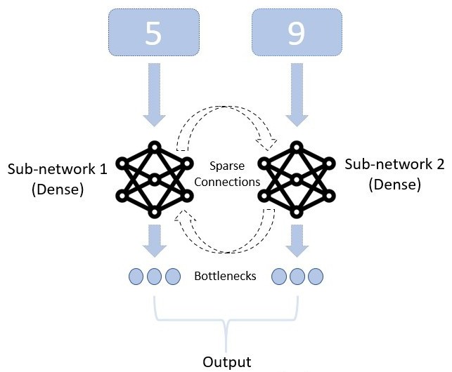
We use this architecture for the majority of the results shown. For one of the functional modularity measures, we introduce an additional bottleneck layer \(\mathbf{b}^{(n)}\) in each sub-network . This bottleneck is composed of an extra, small hidden layer of 5 neurons between the sub-network and the readout (2). In that case, the connection from state to output decomposes in weight matrices \(W^{(n)}_{hb}\), \(W^{(n)}_{br}\) and biases \(\beta^{(n)}_{hb}\), \(\beta^{(n)}_{br}\), and the equations become: \[\begin{aligned} \mathbf{b}^{(n)}&=W^{(n)}_{hb}\mathbf{h}^{(n)}_T+\beta^{(n)}_{hb} \\ \mathbf{r}^{(n)}&=W^{(n)}_{br}\mathbf{b}^{(n)}+\beta^{(n)}_{br}.\end{aligned}\]
In all cases, weights are initialized following a uniform distribution \(\mathcal{U}(-0.1, 0.1)\)
Structural modularity
We define the fraction of connections between two sub-networks as \(p\in[1/N^2,1]\). The same fraction of connections is used in each direction. The smallest value is \(p=1/N^2\) corresponding to a single connection in each direction, and the largest fraction \(p=1\) corresponds to \(N^2\) connections in each direction (all-to-all connectivity).
We adapt the \(Q\) metric for structural modularity (Newman 2006) to a directed graph: \[\label{eq:Q-def} Q = \frac{1}{M}\sum_{ij}(A_{ij}-P_{ij})\delta_{g_ig_j},\] where \(M\) is the total number of edges in the network, \(A\) is the adjacency matrix, \(\delta\) is the Kronecker delta, \(g_i\) is the group index of node \(i\), and \(P_{ij}\) is the probability of a connection between nodes \(i\) and \(j\) if we randomized the edges respecting node degrees. For our network, we can analytically compute (6): \[\label{eq:Q} Q=\frac{1}{2}\cdot\frac{1-p}{1+p}.\] This varies from \(Q=0\) when \(p=1\) (all nodes connected, so no modularity) to \(Q=1/2\) for \(p=0\) (no connections between the sub-networks, so perfect modularity). Note that for \(g\) equally sized groups in a network, the maximum value that \(Q\) can attain is \(1-1/g\).
Training
The sub-networks are trained with gradient descent using the ADADELTA (Zeiler 2012) optimizer. The sparse connections in-between sub-networks are trained using the Deep-R algorithm (Bellec et al. 2018). Each weight is assigned a constant sign \(s_{ij}\) and a associated parameter \(\phi_{ij}\). Any weight \(w_{ij}\) is considered active only if the corresponding parameter \(\phi_{ij} >0\). If not the weight is said to be dormant. For non-negative \(\phi_{ij}\), the corresponding weight is thus given by \(w_{ij} = s_{ij}\phi_{ij}\). For others, weights are set to 0. Ensuring sparsity of the weight matrix comes from ensuring that only the desired number of values of \(\mathbf{\phi}\) are positive at all times. We start with the desired number of positive parameters based on the sparsity \(p\), picked at random. Only those parameters then undergo a gradient descent step, using a separate ADAM optimizer (Kingma and Ba 2017), followed by a random walk step. Whenever one of these becomes negative, effectively setting its weight to 0, we pick at random a new one to become positive. This ensures that only the desired number of weights is active at all times. The gradient descent reinforces important weights by increasing their corresponding parameters. The random walk in parameter space continuously explores possible connection patterns and allows the network to ’rewire’ in case of changing objectives. Effectively, the parameter responsible for the random walk is annealed from its initial value to 0 when \(p\) goes from 0 to 1. Note that our results are not substantially changed if we remove the random walk exploration but we found that Deep-R greatly improves performances at very high sparsities.
Functional modularity
Defining functional modularity is challenging. We want to capture the notion that a sub-network is capable of doing a sub-task independently, which we call functional specialization. However, if that network has never been trained directly on the sub-task, and has always had input from neurons outside the sub-network, it is unlikely to be able to do so without some re-training, which changes the function of the sub-network. We considered three ways of addressing this issue, leading to three quantitative measures of specialization, described below. None of the measures are, individually, entirely satisfactory. However, we show in 4 that all three measures qualitatively agree, suggesting that despite potential individual problems with these measures, they are measuring something meaningful.
We first define three separate metrics, and then give a standard normalization to turn them into comparable specialization measures in 3.4.
Bottleneck metric
One straightforward approach to measuring specialization of a sub-network on a particular sub-task would be to directly evaluate how well it performs on that sub-task. In our case, that would be monitoring individual performance of sub-networks when asked to predict either their own or the other sub-network’s corresponding digits. However, without modification of the network, the sub-networks would continue to predict digits based on the global parity as they were initially trained to do. Re-training only the linear readout of sub-networks while leaving the recurrent weights fixed allows for good performance on this sub-task. However, due to the simplicity of the task, re-training the whole hidden state to output readout is sufficiently powerful to allow for excellent performance even if the recurrent weights are random and untrained, so this cannot measure anything meaningful about the trained weights. The issue is that the full state of the sub-network contains a large amount of information about the original stimulus, and not just the result of any computations carried out by the sub-network, which is the part we are interested in.
To effectively constrain the amount of information readily available to the readout layer, we introduced a narrow bottleneck of only 5 neurons in the architecture, between the sub-network and the readout (2). The state of the bottleneck neurons is sufficient to carry all the information about the digit class but insufficient to represent much information about the stimulus itself. Re-training the bottleneck-output readout then provides us with a measure of performance of the sub-network on the sub-task of classifying the digit. This approach was inspired by the concept of the information bottleneck (Tishby and Zaslavsky 2015) as it minimizes the mutual information between the bottleneck state and the stimulus, while maximizing the mutual information between the bottleneck state and the digit class.
Concretely, for sub-network \(n\) on sub-task \(k\), the bottleneck metric \(\mathcal{M}(n,k)\) is the mean accuracy after:
Training the network on the main task.
Freezing all parameters except the weights \(W_{br}^{(n)}\) and biases \(\beta_{br}^{(n)}\) between the bottleneck and readout of sub-network \(n\).
Re-initializing and retraining only those weights and biases on the task of recognizing digit \(k\).
Weight mask metric
Another promising approach to measure specialization comes from the recently discovered idea of weight masking. In order to determine which weights contribute to which part of the overall computation of a network, a binary mask is applied onto the network’s weights, effectively setting most of them to 0. This mask is trained to maximize performance of the masked network on a target objective, while the actual values of weights remain frozen. This idea was applied to find high performing sub-networks of randomly initialized networks (Frankle and Carbin 2019; Ramanujan et al. 2020) and more recently to quantify functional modularity (Csordás, Steenkiste, and Schmidhuber 2021). Our method is similar to this latter approach but uses a different algorithm (Ramanujan et al. 2020) to train and discover the masks, and does not exploit the resulting masks in the same manner. The masks are trained as follows: each weight is fixed but is attributed a differentiable score, with only the top \(q\%\) scoring weights being used in the forward pass. The training of the mask consists of adjusting those scores to maximize the performance of the masked network on the desired objective. Once a mask is discovered for a particular sub-task, the analysis of the performance of the masks, what weights are retained and the attributions of those weights among the sub-networks serve as metrics for specialization.
It should be noted that binary weight masks can be used to discover high performing sub-networks even in randomly initialized networks (supermasks). We verified that the performance of the discovered masks were substantially better when applied to already trained networks, confirming that these could indeed be used to measure specialization.
The weight mask metric of sub-network \(n\) on sub-task \(k\) is the proportion of weights, after training of the weight mask on predicting digit \(k\), that are present in sub-network \(n\). Let \(\theta=\theta^0\cup\theta^1\) to be the set of parameters of the whole network trained on the full task, where \(\theta^n\) are the parameters in sub-network \(n\). We define \(\mathcal{S}^{q}_k\subseteq\theta\) to be the subset of parameters selected by a mask trained on predicting digit \(k\) using only \(q\%\) of parameters from \(\theta\). The weight mask metric is then defined as follows, where \(|\cdot|\) indicates cardinality: \[\mathcal{M}(n, k) = \frac{|\mathcal{S}^{q}_k\cap\theta^n|}{|\mathcal{S}^{q}_k|} = \frac{|\mathcal{S}^{q}_k\cap\theta^n|}{q|\theta|}\]
In this work, the weight mask is not applied to input weights \(W_{ih}\) and biases \(\beta_{ih}\). We chose \(q\) to be as high as possible while ensuring \(\mathcal{M}(n, n) = 1\) in the most extreme case of sparsity. In our case, this led to selecting 5% of the total model’s weights, \(q = 0.05\). We also ensured that this value still led to good performance in the masks discovered.
Correlation metric
Our final approach is to directly examine hidden layers’ activities, and how each sub-network’s activity depends on each digit. One way of doing this is to examine the correlation of hidden states of sub-networks when only varying a single digit out of the input pair. A sub-network highly specialized on its corresponding digit should exhibit high correlation between states corresponding to inputs where only the second, irrelevant digit is varying. To measure the correlation we simply used the mean Pearson correlation coefficient.
For sub-network \(n\) on sub-task \(k\), we compute the mean Pearson correlation coefficient between the hidden states of sub-network \(n\) for pairs of examples \(x\) and \(x^\prime\) where digit \(k\) of the two examples is the same. Writing \(\mathop{\mathrm{corr}}(x,y)\) for the Pearson correlation coefficient of vectors \(x\) and \(y\):
\[\mathcal{M}(n, k)=\mathbb{E}_{x, x^\prime}[\;\mathop{\mathrm{corr}}(h_n(x), h_n(x^\prime)\;|\;\mbox{digit $k$ of $x$ $=$ digit $k$ of $x^\prime$}\;].\]
Specialization Measure
We have now defined our three metrics. Each of those is applied to each sub-network for each sub-task. We write \(\mathcal{M}(n, k)\) for a metric of sub-network \(n\) on task \(k\). Our specialization measure is then defined as
\[\mathcal{M}_{spec}(n) = \frac{\mathcal{M}(n,n)-\mathcal{M}(n,1-n)}{\mathcal{M}(n,n)+\mathcal{M}(n,1-n)}.\]
So \(\mathcal{M}(n,n)\) is sub-network \(n\) on the task of recognizing its own digit, and \(\mathcal{M}(n,1-n)\) is sub-network \(n\) recognizing the digit of the other sub-network. This specialization measure can range from 1, which corresponds to a fully specialized sub-network on its corresponding sub-task, to -1, which indicates full specialization on the other sub-network’s corresponding sub-task.
Results
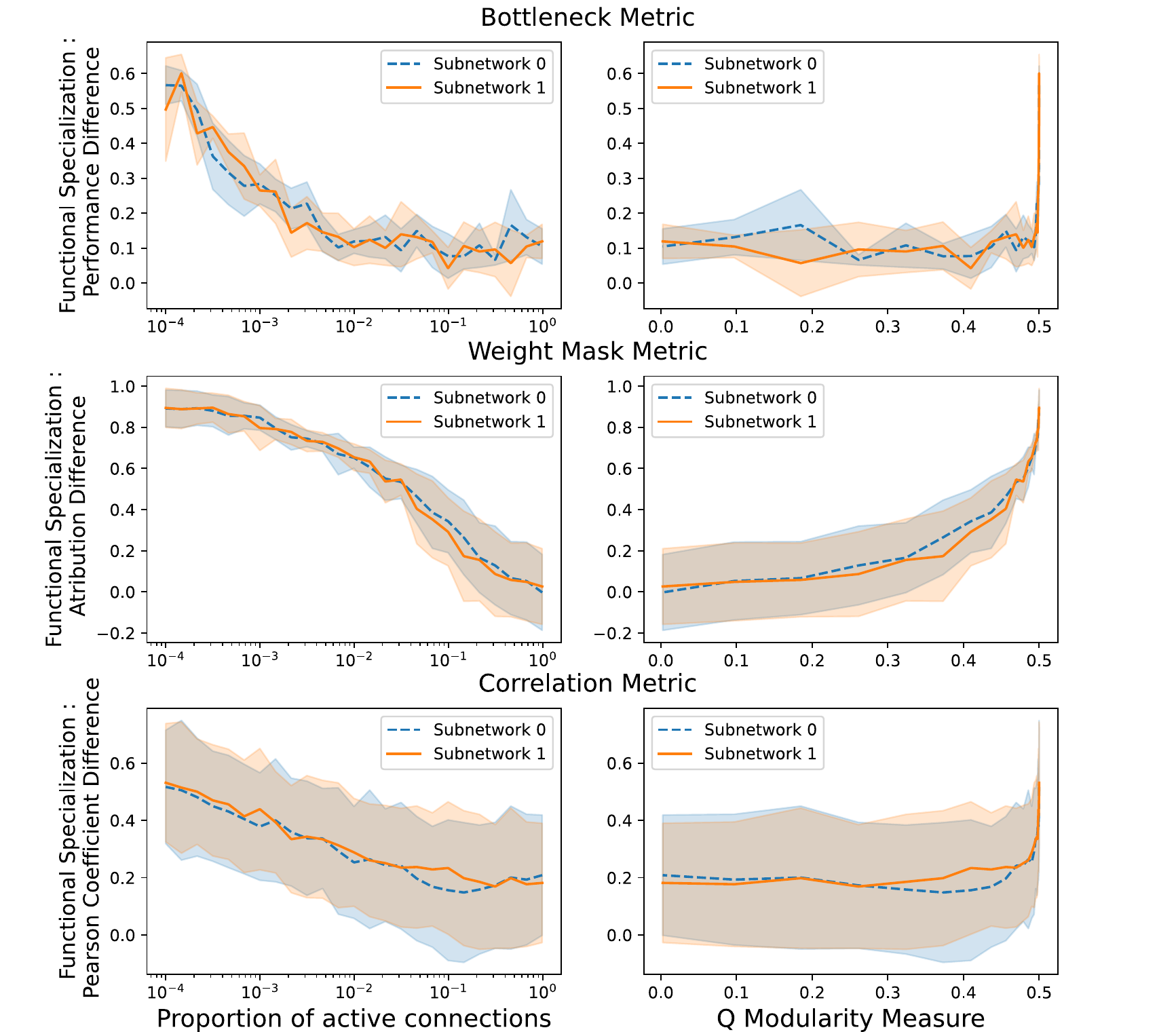
shows how each of the three measures of functional specialization discussed in 3 varies with the structural modularity of the network, measured either with the sparsity \(p\) (left) or with the \(Q\) modularity measure (right). In each case, the qualitative pattern is the same: a sparser, more structurally modular network leads to a greater degree of functional specialization. This is reassuring in two senses.
Firstly, it shows that our three very different measures of functional specialization qualitatively agree, suggesting they are measuring something meaningful. Secondly, it shows that as we would hope, imposing structural modularity is sufficient to induce functional modularity.
However, we also note that only extreme levels of sparsity or structural modularity lead to a high degree of functional specialization across all three measures. For the bottleneck and correlation metrics, we require \(Q>0.49\) (or sparsity \(p<0.01\)) before we start to see a rise in functional specialization. Note that the highest value possible for \(Q\) is 0.5 when there are only two equally-sized sub-networks. This trend is less extreme for the weight mask metric, where we start to see a rise from the start, but functional specialization according to this measure still depends strongly non-linearly on structural modularity, without substantially increasing until around \(Q>0.4\) (\(p<0.11\)).
In other words, across all measures, a high degree of structural modularity (e.g. \(Q=0.35\)) is consistent with little to no functional specialization.
Discussion
We have demonstrated two substantial results. The first is that, by using a carefully hand crafted example it is possible to systematically relate structural and functional modularity. We showed that three entirely different measures of functional specialization qualitatively agree in this case. This allows us some confidence that these measures do reflect an important underlying property of these networks, even if individually they have limitations (see below). Furthermore, each measure of functional modularity increases monotonically with increasing levels of structural modularity. This reassuringly matches our intuition.
The second result, however, is that we require a very high degree of structural modularity to ensure functional modularity. Or, put another way, a moderately high degree of structural modularity can be seen in a network that has almost no functional modularity whatsoever. This has implications both for the design of artificial networks and for the analysis of biological networks.
For designing networks, it means that imposing a moderate degree of structural modularity is unlikely to be sufficient, on its own, to ensure any degree of functional modularity. If we want functional modularity, we either need to use extreme levels of structural modularity, imposed via very sparse connections between sub-networks, or – perhaps better – we need to use other methods to induce this functional modularity.
In terms of analyzing biological data, our results demonstrate that we should not conclude any degree of functional modularity simply by observing a moderate degree of structural modularity. This potentially poses problems for approaches such as connectomics (Sporns, Tononi, and Kötter 2005), which assume that knowing the structural properties of networks will give us good constraints on their functional properties.
Despite good qualitative agreement between the measures of functional modularity, each one individually has significant limitations individually. In both bottleneck and weight-mask measures, for example, we effectively retrain part of the network to perform a sub-task, and this training requires making choices of parameters such as learning rate, number of epochs, etc. The resulting metric depends on these choices.
Another limitation of our findings comes from the task design. In order to easily witness and measure specialization, we designed a simple global task that could decompose into sub-tasks. The information that needs to be transmitted between the sub-networks, however, is minimal (a single bit). This could explain why we only see specialization at extreme levels of sparsity. An interesting future work would be to craft a global task where the amount of information transmission needed among sub-networks in order to solve the task could be independently controlled. We could then examine how the relationship between sparsity (structural modularity) and specialization (functional modularity) depends on the required communication bandwidth. Would it shift, but preserve the overall pattern?
In the end modularity is really like beauty in art. If you give it time, and different perspectives, you can start to discern its ever-changing shape.
Appendix
Q measure derivation
(Newman 2006) defines the modularity measure \(Q\) for an undirected graph. We modify the definition for a directed graph as: \[ Q = \frac{1}{M}\sum_{ij}(A_{ij}-P_{ij})\delta_{g_ig_j} = \frac{1}{M}\sum_{ij}\left(A_{ij}-\frac{k_i^{out}k_j^{in}}{M}\right)\delta_{g_ig_j}\] where \(M\) is the total number of edges in the network, \(A\) is the adjacency matrix, \(\delta\) is the Kronecker delta, \(g_i\) is the group index of node \(i\), \(k_i^{out}/k_j^{in}\) are the out-degree/in-degree of node \(i/j\) respectively, used to compute \(P_{ij}\): the probability of a connection between nodes \(i\) and \(j\) if we randomized the edges respecting node degrees. For our network, we have 2 sub-networks (with group index 0 and 1 respectively) of N neurons, densely connected, with p% active inter-connections between the two. From this we get: \[\begin{aligned} &M = 2N^2(1+p) \\ &\forall i \in [1, 2N], \quad g_i = \begin{cases} 0,& \text{if } i \in [0, N-1]\\ 1, & \text{if } i \in [N, 2N] \end{cases} \\ &\forall(i,j) \in [0, 2N]^2, \quad A_{i,j} = \begin{cases} 1,& \text{if } \delta_{g_ig_j} = 1\\ 0 \text{ or } 1, & \text{if } \delta_{g_ig_j} = 0 \end{cases} \\ &\forall(i,j) \in [0, 2N]^2, \quad \begin{cases} k_i^{out} = \sum_{j'}A_{ij'} \approx N(1+p) \\ k_j^{in} = \sum_{i'}A_{i'j} \approx N(1+p) \end{cases} \\ \text{And} \quad &\begin{cases} \sum_{i}k_i^{out} = \sum_{i}\sum_{j'}A_{ij'} = N^2(1+p) \\ \sum_{j}k_j^{in} = \sum_{j}\sum_{i'}A_{i'j} = N^2(1+p) \end{cases} \\ \text{Thus : } &Q = \frac{1}{2N^2(1+p)}\sum_{ij}\left (A_{ij} - \frac{(1+p)}{2}\right)\delta_{g_ig_j} \\&Q= \frac{1}{2N^2(1+p)}(2N^2)\left(1 - \frac{(1+p)}{2}\right) \\ &\boxed{Q= \frac{1-p}{2(1+p)}}\end{aligned}\]
Training parameters
Here we present all training parameters used in the global model training (parity task), the discovery of the weight masks and the bottleneck-readout retraining. When two optimizers or learning rates are specified, they correspond to the parameters for the sub-networks/sparse-connections respectively. When a parameters is indicated as a range, it was geometrically decreased in between the two bounds when inter-connections sparsity spanned from 0 to 1. In the case of the global training, we had to train both architectures ([fig:archi,fig:bottleneck-archi]), we thus indicates parameters (bottleneck size and number of epochs) for the absence/presence of the bottleneck.
| Global training | Mask training | Bottleneck re-training | |
|---|---|---|---|
| Number of sub-networks | \(2\) | \(2\) | \(2\) |
| Number of input neurons | \(2*784\) | \(2*784\) | \(2*784\) |
| Number of hidden neurons | \(2*100\) | \(2*100\) | \(2*100\) |
| Bottleneck size | -/5 | - | \(5\) |
| Number of classes | \(10\) | \(10\) | \(10\) |
| Number epochs | \(5/7\) | \(1\) | \(5\) |
| Optimizer | Adadelta/Adam | SGD | Adadelta |
| Learning rate | \(0.5/[0.1-0.01]\) | \(0.1\) | \(0.5\) |
| Betas | \(0.9/0.95\) | - | \(0.9\) |
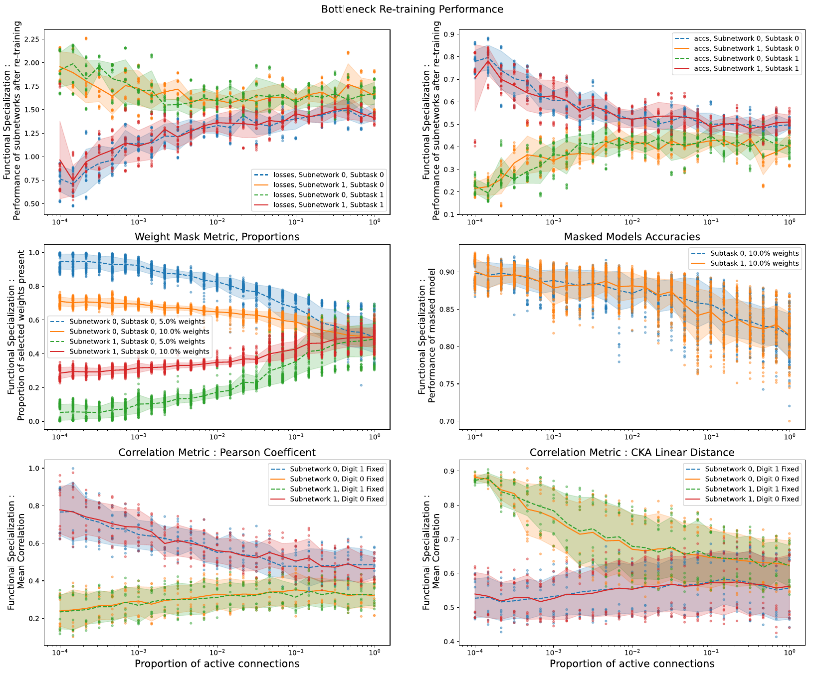
Raw metrics
In order to measure specialization, we used a normalized difference between sub-tasks over three different metrics. This difference however isn’t a fool-proof way to arrive at out measure. No matter the raw performance of a sub-network for a given metric, if it achieves the same for both sub-tasks then our specialization measure is equal to 0. The question that a sub-network performing perfectly for both sub-task should get the same measure as one performing very poorly on both is thus open. Fortunately this was not the case as shown in the raw metrics (4), and the quantity we measured is meaningful. We also show the results of the correlation metric when using the CKA distance (Kornblith et al. 2019) (note that this metric is defined as a distance, i.e. 0 when highly correlated).
Global model performance
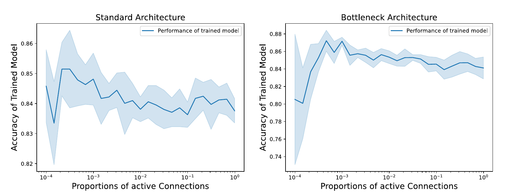
In this study, we measure the specialization of sub-networks for varying sparsity of inter-connections. It is to be noted that this specialization depends on the overall performance of the global model, which in turns should depend on said sparsity of connections. We made sure that every trained model showed good performance so that measures on functional modularity were meaningful (5).
Click to pin
Click to unpin